Formation Control
12 Dec 2019
Post Tags
ROS Robotics Localization Formation-controlTable of Content
This formation control project is my master thesis topic, which controls robots forming a pattern when driving along a desired direction.
Before introduce the algorithm and implementation method, lets see the video of my robots:
1. Formation Control
Formation control generally refers to the control approach to accomplish a specific pattern with a group of robots. It is the foundation of autonomous cooperative control with multi-robots, which can be widely used in surveillance, distributed manipulation, and transportation of large objects. Researchers have developed several methods to solve formation problem, which includes: leader-follower approach, virtual structure, behaviour control, and ect. However, I implemented a decentralized control method using gradient descent algorithm which refers the consensus control
1.1. Dynamic model of vehicles
The dynamical model of vehicles plays a crucial role in the formation control problem. In real world vehicle systems, there are different types of vehicle models, like holonomic model, nonholonomic vehicle model, Euler-Lagrange vehicle model, and high-order dynamic model.
In holonomic vehicle systems, the motion of a vehicle in every axis is independent with each other. Thus, the vehicles can directly go to any position without constraints. The general expression of a holonomic vehicle is
\[\begin{equation} \label{holonomic_equ} \dot{p}_{i}=v_{i}, \quad \dot{v}_{i}=u_{i}, \quad i \in\{1, \ldots, N\} ......(1.1.1) \end{equation}\]Where $p_{i}, v_{i} \in \Re^{n}$ ,$n \in {2,3}$, are the position and the velocity vectors of vehicles. $u_{i}$ is the acceleration input of the vehicles.
For nonholonomic models, the model on $\Re^{2}$ is generally given by
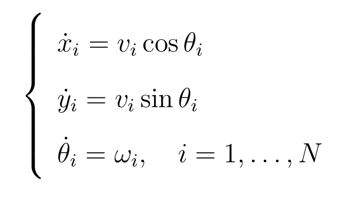 <p> Equation (1.1.2). nonholonomic dynamic model</p></div>
Where the $v_{i}$, ${\theta_i}$ and $\omega_{i}$ are linear velocity, handing direction and angular velocity respectively. The vehicle position in world frame is presented by $p_{i}=|x_{i}, y_{i}|^{\top} \in \Re^{2}$. A general illustration of nonholonomic vehicle model is shown in Fig below.
<p> Equation (1.1.2). nonholonomic dynamic model</p></div>
Where the $v_{i}$, ${\theta_i}$ and $\omega_{i}$ are linear velocity, handing direction and angular velocity respectively. The vehicle position in world frame is presented by $p_{i}=|x_{i}, y_{i}|^{\top} \in \Re^{2}$. A general illustration of nonholonomic vehicle model is shown in Fig below.
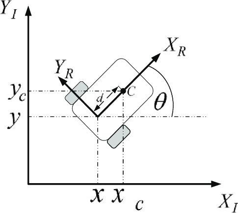 <p> Fig illustration of nonholonomic vehicles.</p></div>
1.2. Gradient descent control
Gradient formation controllers are based on the gradient descent optimization algorithm, which can find the minimum of a function by using iteration methods. For a general formation control case, consider the formation of $\textbf{n}$ vehicles with typical holonomic dynamic, and a graph pattern $\mathscr{G}$. Between arbitrary two vehicles has an edge $\mathscr{E_{ij}}$ where a corresponding potential function (cost function) $V_{ij}$ can be constructed. When these two vehicles are at the desired relative position, the potential function $V_{ij}$ gets the global minimum value. A typical potential function $V_{ij}$ could have the following conditions[1].
\[\begin{equation} \label{con1} V_{i j} : R^{m} \rightarrow R_{ \geq 0} \text{ is continuously differentiable} ......(1.2.1) \end{equation}\] \[\begin{equation} \label{con2} V_{ij}=0 \Longleftrightarrow\left\|p_{i}-p_{j}\right\|=d_{ij} ......(1.2.2) \end{equation}\] \[\begin{equation} \label{con3} \nabla_{p_{i}} V_{ij}=0 \Longleftrightarrow\left\|p_{i}-p_{j}\right\|=d_{ij} ......(1.2.3) \end{equation}\]Where the $d_{ij}$ is the desired relative position between the vehicle $\textbf{i}$ and vehicle $\textbf{j}$. $\nabla_{x}$ is defined as $\nabla_{\boldsymbol{x}} \triangleq\left[\frac{\partial}{\partial x_{1}}, \dots, \frac{\partial}{\partial x_{m}}\right]^{T}$, in 2D case $\nabla_{p_i} = \left[\frac{\partial}{\partial x_{i}}, \frac{\partial}{\partial y_{i}}\right]^{T}$. To calculate all the edges inside the graph, the potential function can be defined as :
\[V = \sum_{(i, j) \in \mathcal{E}(t)} V_{i j} ......(1.2.4)\]Thus, a gradient descent controller for each vehicle can be defined as:
\[\begin{equation} \label{holonomic_ui} u_{i}=-\nabla_{p_{i}}\sum_{(i, j) \in \mathcal{E}(t)} V_{i j} ......(1.2.5) \end{equation}\]It has been proved in article[2] that the formation will finally converge to the desired pattern $\mathscr{G}^f$. If all the conditions (1.1), (1.2), (1.3) are satisfied.
The above conclusion is the basic of gradient formation control algorithm. It will be much complicated to drive a group of robots or vehicles with nonholonomic or other dynamic vehicle model. The method and proof of nonholonomic formation can be found in my thesis[3].
2. Implementation of a formation system
2.1. Overview of the system
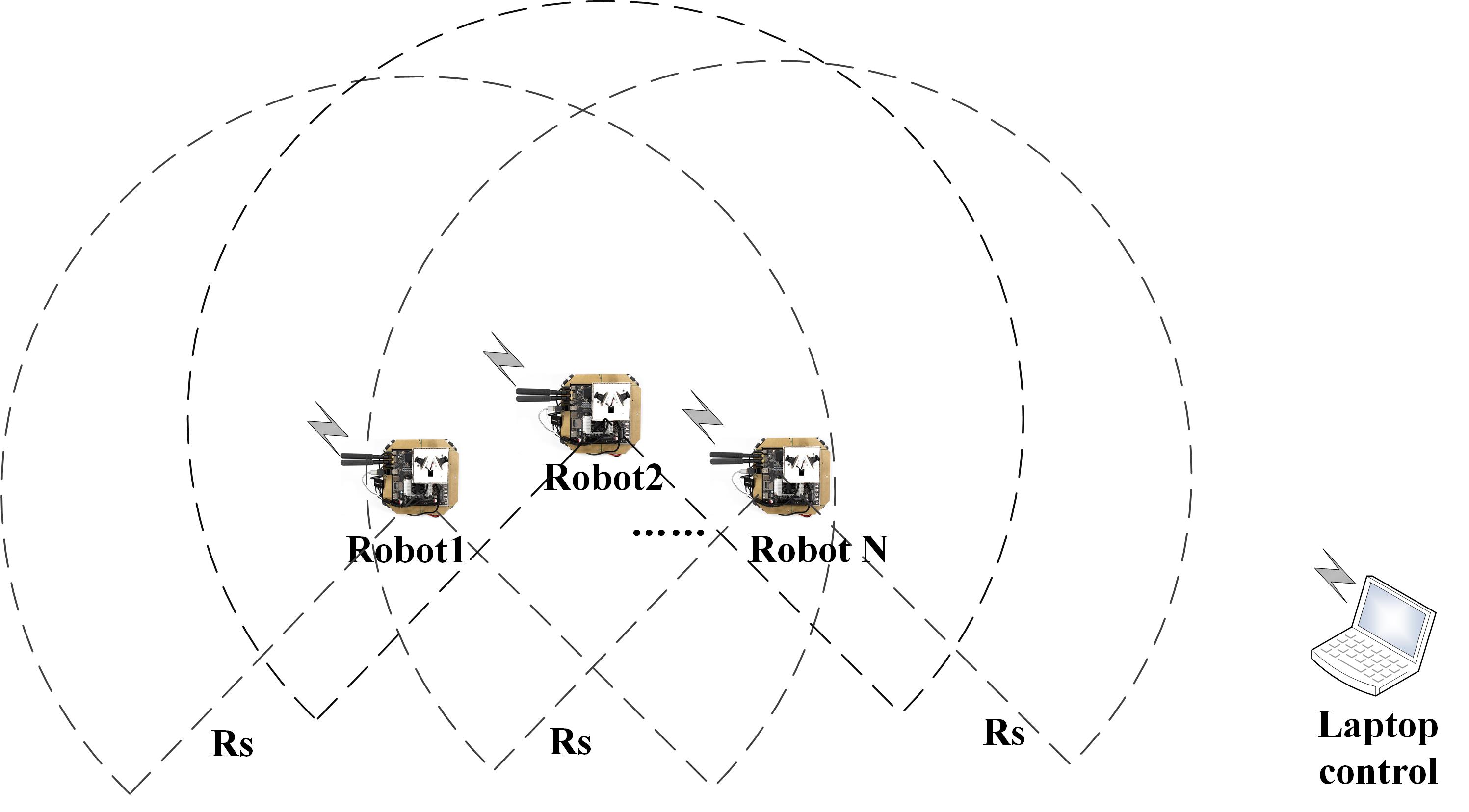
Even it is a distributed control system, we still need a central controller(laptop) to send start and stop command only.
 <p>
<p>
Fig Formation system of 4 vehicles .</p></div>
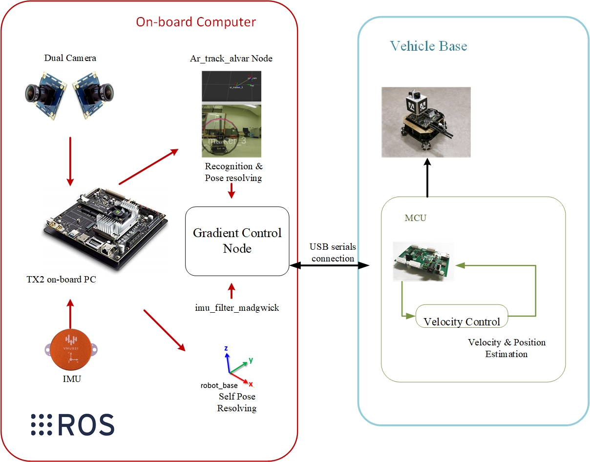
Vehicles are designed by myself with nvida TX2 as high level cointroller, and a stm32f1 based low level controller which used to control motors directly. The picture below is a general architecture that briefly illustrate the main components used in this project. The main program runs on NVIDIA TX2 with Linux system. Robot Operation System (ROS) are used to fulfill high-level action which finally send the desired velocity to the MCU (Micro Controller Unit). MCU is responsible for low-level motors control.
 <p>
<p>
Fig Project Architecture .</p></div>
2.2. Perception – Vision
It is crucial for robot to know where are they and their companions. Basically, people have developed several indoor localization method, like ultrasonic, lidar, vision, and etc. In this project, I use vision, QR-code marker, combined with inertial. For how to use the QR-code I wrote in another post
The vehicles around with 4 markers, and attached with 2 cameras in opposite direction to localize each other.
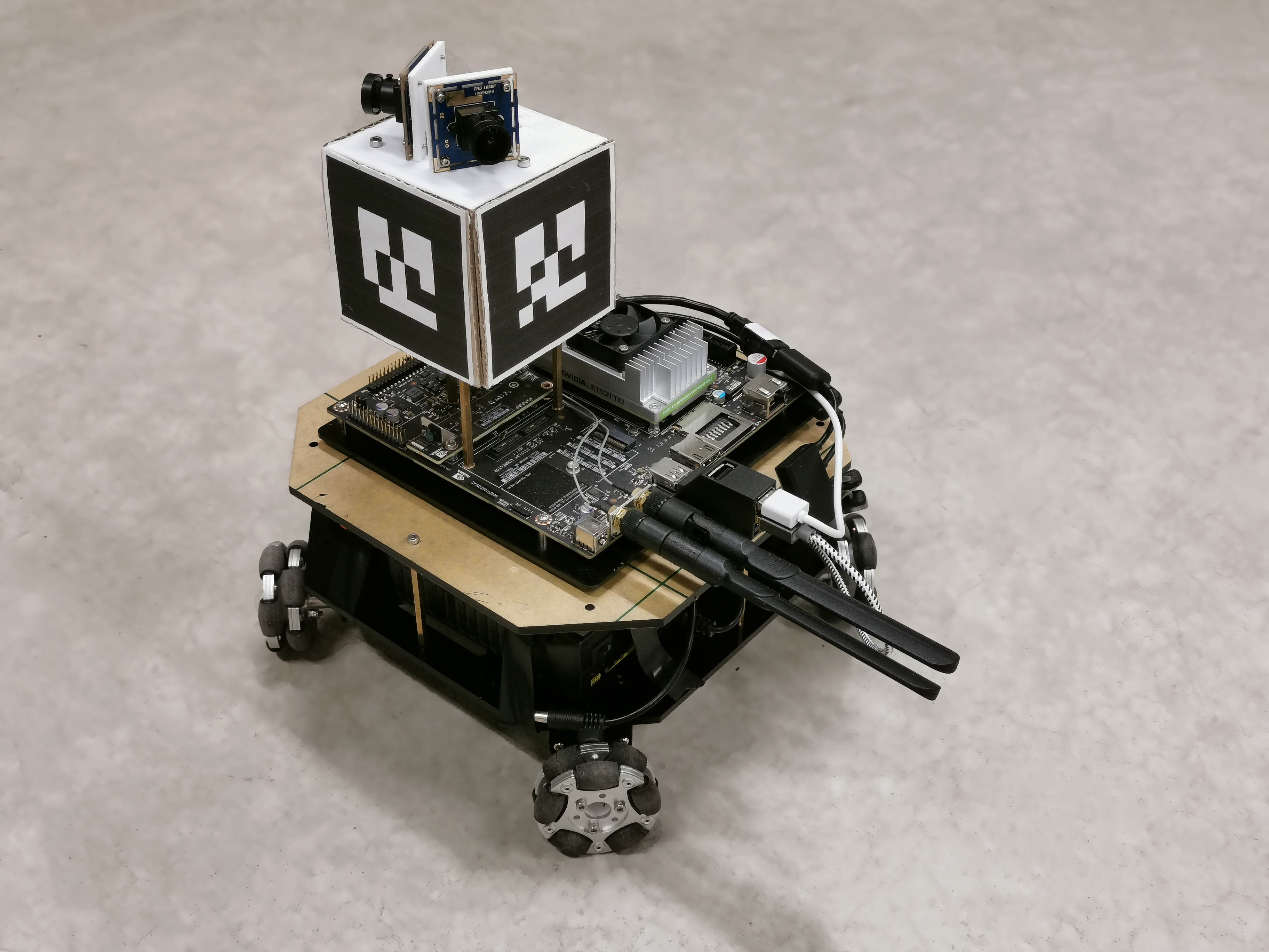 <p>
<p>
Fig Photo of the vehicle .</p></div>
2.3. Code and design
/* TODO */
The code can be found in github